Assets with in-memory computations

So far when writing assets, you’ve orchestrated computations in a database and did some light work in Python, such as downloading a file. In this section, you’ll learn how to use Dagster to orchestrate Python-based computation by using Python to generate and transform your data and build a report.

Creating metrics using assets

Having all of your assets in one file becomes difficult to manage. Let’s separate the assets by their purpose and put these analysis-focused assets in a different file than the assets that ingest data.

1. In the assets directory, navigate to and open the metrics.py file.

2. At the top of the assets/metrics.py file, add the following imports:

   from dagster import asset
   
   import plotly.express as px
   import plotly.io as pio
   import geopandas as gpd
   
   import duckdb
   import os
   
   from . import constants
   

   There may be some imports you’re unfamiliar with, but we’ll cover those as we use them.

3. Next, define the manhattan_stats asset and its dependencies. Copy and paste the following code to the end of metrics.py :

   @asset(
       deps=["taxi_trips", "taxi_zones"]
   )
   def manhattan_stats() -> None:
   

4. Now, let’s add the logic to calculate manhattan_stats. Update the manhattan_stats asset definition to reflect the changes below:

   @asset(
       deps=["taxi_trips", "taxi_zones"]
   )
   def manhattan_stats() -> None:
       query = """
           select
               zones.zone,
               zones.borough,
               zones.geometry,
               count(1) as num_trips,
           from trips
           left join zones on trips.pickup_zone_id = zones.zone_id
           where borough = 'Manhattan' and geometry is not null
           group by zone, borough, geometry
       """
   
       conn = duckdb.connect(os.getenv("DUCKDB_DATABASE"))
       trips_by_zone = conn.execute(query).fetch_df()
   
       trips_by_zone["geometry"] = gpd.GeoSeries.from_wkt(trips_by_zone["geometry"])
       trips_by_zone = gpd.GeoDataFrame(trips_by_zone)
   
       with open(constants.MANHATTAN_STATS_FILE_PATH, 'w') as output_file:
           output_file.write(trips_by_zone.to_json())
   

   Let’s walk through the code. It:

   1. Makes a SQL query that joins the trips and zones tables, filters down to just trips in Manhattan, and then aggregates the data to get the number of trips per neighborhood.
   2. Executes that query against the same DuckDB database that you ingested data into in the other assets.
   3. Leverages the GeoPandas library to turn the messy coordinates into a format other libraries can use.
   4. Saves the transformed data to a GeoJSON file.

Materializing the metrics

Reload the definitions in the UI, and the manhattan_stats asset should now be visible on the asset graph. Select it and click the Materialize selected button.

After the materialization completes successfully, verify that you have a (large but) valid JSON file at data/staging/manhattan_stats.geojson.

Making a map

In this section, you’ll create an asset that depends on manhattan_stats, loads its GeoJSON data, and creates a visualization out of it.

1. At the bottom of metrics.py file, copy and paste the following:

   @asset(
       deps=["manhattan_stats"],
   )
   def manhattan_map() -> None:
       trips_by_zone = gpd.read_file(constants.MANHATTAN_STATS_FILE_PATH)
   
       fig = px.choropleth_mapbox(trips_by_zone,
           geojson=trips_by_zone.geometry.__geo_interface__,
           locations=trips_by_zone.index,
           color='num_trips',
           color_continuous_scale='Plasma',
           mapbox_style='carto-positron',
           center={'lat': 40.758, 'lon': -73.985},
           zoom=11,
           opacity=0.7,
           labels={'num_trips': 'Number of Trips'}
       )
   
       pio.write_image(fig, constants.MANHATTAN_MAP_FILE_PATH)
   

   The code above does the following:

   1. Defines a new asset called manhattan_map, which is dependent on manhattan_stats.
   2. Reads the GeoJSON file back into memory.
   3. Creates a map as a data visualization using the Plotly visualization library.
   4. Saves the visualization as a PNG.

2. In the UI, click Reload Definitions to allow Dagster to detect the new asset.

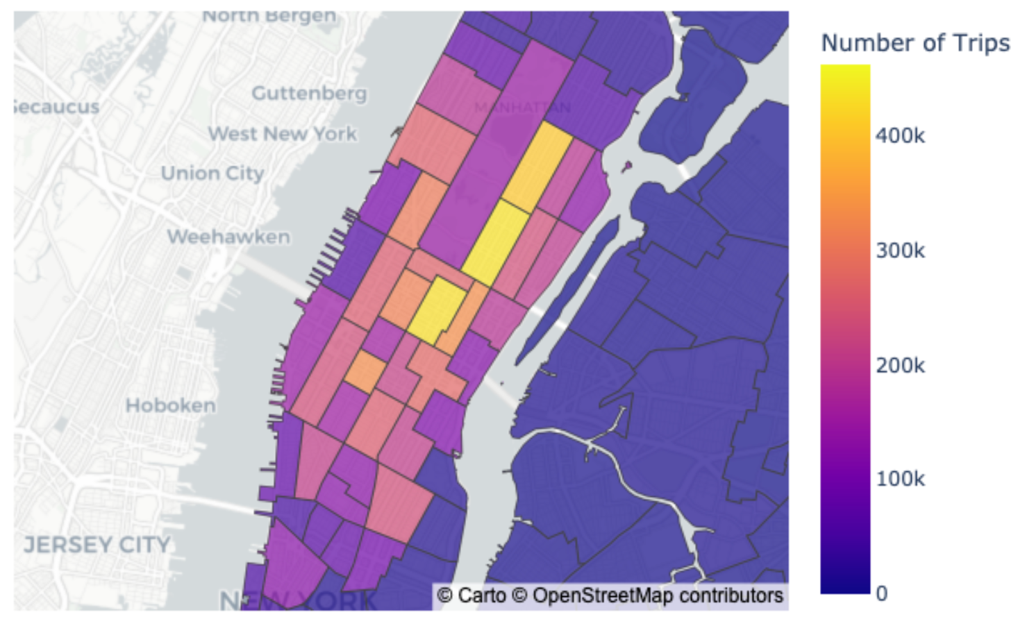
3. In the asset graph, select the manhattan_map asset and click Materialize selected.

4. Open the file at data/outputs/manhattan_map.png to confirm the materialization worked correctly. The file should look like the following: